Simulating protein domain evolution with a cellular automaton
Abstract
In June 2023 I completed an implementation project for the Computational Genomics seminar at UNAM’s Facultad de Ciencias. It asked how a cellular automaton can simulate the evolution of protein domains, and followed the method of Xiao, Xue, Stamatovic and Qiu (2020): a one-dimensional lattice in which an empty cell next to a filled one draws its state by roulette-wheel selection from two adjacency matrices, F2B and B2F. As a deliberate proof of concept, my notebook estimates both matrices from the 3890 adjacent pairs of the 3891-nucleotide bont gene of Clostridium botulinum, so its states are the bases A, C, G and T. It runs a 17-cell lattice for 8 updates from an ancestral A. The October 2026 re-run reproduces all 32 printed matrix values exactly. The notebook updates the lattice in place, so in all 10000 seeded re-runs the first update filled cells 9 to 15. The project has no evaluation against real domain architectures.
The question
This was my implementation project for the Computational Genomics seminar (Seminario de Genómica Computacional) at UNAM’s Facultad de Ciencias. The final slides, presented in 2023, carry the title Autómatas Celulares en la Simulación de la Dinámica de Dominios Proteicos. The repository holds the 18-page slide deck, a Jupyter notebook with three executed code cells, and one input file in FASTA format.
The slides ask one research question: how can cellular automata be used to simulate the evolution of protein domains? The objective follows from it, to develop a model based on cellular automata that simulates that evolution. The motivation they give is that domain evolution can provide information about the history of life and the function of current organisms, and that it could help anticipate how diseases progress or how pathogens evolve.
The progress deck I committed in April 2023 had a second objective, to analyze and validate the proposed model with experimental data. The final deck in June keeps only the first one.
The method I followed
The slides follow Xiao, Xue, Stamatovic and Qiu (2020), who simulate domain evolution with a one-dimensional probabilistic cellular automaton [1]. As the slides define it, each cell is in one of g + 3 states: g domain classes, two termination symbols and the empty state ∅. At the start, the central cell holds an ancestral domain and every other cell is empty. The automaton evolves for as many time steps as the number of domains in the protein with the most domains in the training data.
Four rules decide the next state of a cell from the cell and its two neighbors:
- Rule A, inheritance. A filled cell keeps its state.
- Rule B, front-to-back evolution. An empty cell whose left neighbor is filled and whose right neighbor is empty takes a state drawn by roulette-wheel selection from the F2B row of its left neighbor.
- Rule C, back-to-front evolution. The mirror case: an empty cell with an empty left neighbor and a filled right neighbor draws from the B2F row of its right neighbor.
- Rule D, return to inanimation. An empty cell with two empty neighbors stays empty.
F2B[x][y] is the probability that state y follows state x, and B2F[x][y] is the probability that y precedes x. Both come from counting adjacent pairs in the training data.
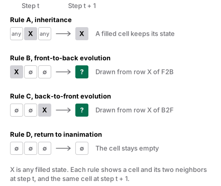
The slides also present Margaret Dayhoff’s amino-acid substitution matrix as a model the project would use [3]. The notebook doesn’t use it.
What the notebook implements
The input is DNA
The notebook reads line 2 of src/protein.fasta into a variable named secuencia_proteina (“protein sequence”). The file holds a nucleotide sequence. Using one was a deliberate design choice: the notebook is a proof of concept of the method on a nucleotide sequence, with the four bases in the role of domain classes. Its header is:
>NC_009495.1:909709-913599 bont [organism=Clostridium botulinum A str. ATCC 3502] [GeneID=5185061] [chromosome=]
The October 2026 re-run counted 3891 characters, all of them A, C, G or T: A 1579, C 394, G 629 and T 1289. That length is 913599 − 909709 + 1. Translated with Biopython 1.85 (genetic code table 11), the sequence gives 1297 codons with a single stop codon at the end, and the protein begins MPFVNKQFNYKDPVNGVDIAYIKIPNAGQMQPV. So the file is the coding sequence of the bont gene (botulinum neurotoxin). The notebook never translates it, and the four states the automaton evolves are the bases A, C, G and T.
The matrices
The first cell counts every adjacent pair (s[i], s[i+1]) of the sequence, 3890 pairs in all, and divides each row of counts by its total. The result is F2B[x][y] = P(next base is y | current base is x) and B2F[x][y] = P(previous base is y | current base is x).
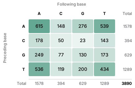
For example, the notebook prints F2B AA as 0.3897338403041825, which is 615/1578, and B2F “CA” (C before A) as 0.11280101394169835, which is 178/1578.
The automaton
The second cell defines the class AutomataCelular(m, g, dominio_ancestral, F2B, B2F). It builds a lattice of 2m + 1 cells set to '∅' and places the ancestral state in cell m. Roulette-wheel selection draws np.random.uniform(0, sum(p)) and returns the first state whose cumulative probability exceeds the draw. The notebook sets no random seed.
The update loop runs over cells 1 to 2m − 1, so it never updates the first and last cells, and applies rules A to D in that order. It writes each new state into the same array it reads. The third cell runs the automaton with m=8, g=4 and ancestral state 'A': a lattice of 17 cells, 8 updates and 9 printed rows.
The code differs from the slides in five places:
Slides (main.tex) |
Notebook (CA.ipynb) |
|
|---|---|---|
| States | g + 3: domain classes, two termination symbols and ∅ | 5: A, C, G, T and ∅ |
| g | number of domain classes | passed as 4 and never read |
| Number of steps | domains in the protein with the most domains in the training data | m = 8, a constant |
| Update | every rule applies “in the next time step” | in place, from left to right |
| Boundary cells | not stated | cells 0 and 16 never change |
What the re-run measured
Everything in this section comes from the October 2026 re-run, with Python 3.9.6 and numpy 2.0.2. The notebook records Python 3.8.4.
- The notebook was executed unchanged with nbconvert, and its output was compared with the committed output.
- The class was copied into a script that records every step and was run with numpy seeds 0 to 9 twice: once with the notebook’s in-place update and once with a synchronous variant in which every cell reads the previous step, which is what the slides describe.
- The in-place version was run 10000 times from seed 12345, and the filled cells were counted after the first update and at the end, together with the base-pair frequencies on the right side of the lattice.
- The probability of the committed final row was computed under the notebook’s own model.
Results
The run in the notebook
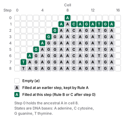
After the first update, cells 7 to 15 are filled. Rule C fills cell 7, and Rule B fills cells 9 to 15 in a single sweep, since when the loop reaches cell 10, cell 9 already holds the base drawn for it a moment earlier. The left side then gains one cell per update and reaches cell 1 at step 7. The last update changes nothing, because cell 0 never updates. The final row is ∅TAGAGGAACAGATGA∅.
The results slide is qualitative. In my translation, it says that “a novel implementation has been shown to represent the evolution of protein domains, taking advantage of the complex nature of cellular automata to reflect with simplicity a phenomenon that is difficult to study and that can be exploited in multiple scientific areas.” It reports no metric, no comparison with real domain architectures and no repeated runs.
The re-run
| Check (re-run) | Result |
|---|---|
| The 16 F2B and 16 B2F values printed by the first cell | byte-identical to the committed output |
| Shape of the unseeded automaton run | different bases, same shape as the committed run |
| First update fills all 7 cells from 9 to 15 (10000 in-place runs) | 10000 of 10000 |
| Filled cells in the final lattice (10000 in-place runs) | 15 in every run |
| Frequency of A after A on the right side, against F2B AA | 0.39031983318159125 against 0.3897338403041825 |
| Probability of the committed final row under the model | 8.073410076915032e-09 |
The last value is the product of 14 factors: 7 F2B values for cells 9 to 15 and 7 B2F values for cells 7 to 1. The committed row is one draw among many.
Discussion
The re-run confirms two parts of the notebook. The matrices match to the last digit, and the base pairs that the roulette wheel draws on the right side follow F2B, for example A after A with frequency 0.39031983318159125 against 0.3897338403041825.
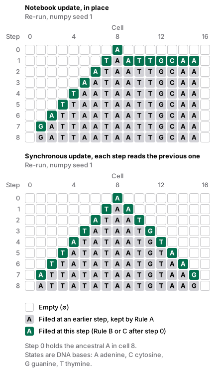
The in-place update changes the order in which cells fill, and it leaves the distribution of the final row unchanged. Reading the code, under both update orders each cell to the right of the center is drawn from the F2B row of its left neighbor, and each cell to the left of the center from the B2F row of its right neighbor. So every final row is two chains of 7 bases drawn outward from the ancestral A, with the adjacent-pair statistics of the bont gene. The two orders differ in the space-time diagram, which is the path the lattice takes over the 8 updates.
For that reason the model, as implemented, says nothing yet about protein domains. By design it is a proof of concept on one nucleotide sequence, with no domain annotation and no training set of proteins; g is never read and the two termination symbols never appear; m is fixed at 8; and the Dayhoff matrix appears only on a slide. The project has no evaluation, and the validation objective from April didn’t reach the final deck.
The references on the slides also have errors. The main citation lists “Qiu, Y., Zhang, X. (2020)”, while the article at that DOI is by Xuan Xiao, Guang-Fu Xue, Biljana Stamatovic and Wang-Ren Qiu [1]. The second reference gives “Q. Rev. Biol. 21:745” for a DOI that resolves to Mathematics of Computation 21(100):745 [2]. None of the five images on the slides states its source, so Figure 1 redraws the rules from the text of the slides.
The slide titled Futuro (future) lists three items. The first says, in the present tense, that the implementation uses protein domains from an established database to generate real structures; the repository contains no such data, so I read it as a planned step. The second proposes running MDAT on real structures and on generated ones to produce values that measure how similar their evolution is [4]. The third is an open question: how feasible are random generation methods for the search of structures?
Reproduce it
These commands run from a fresh clone. They were verified in the October 2026 re-run with Python 3.9.6, numpy 2.0.2, nbconvert 7.17.2 and ipykernel 6.31.0.
git clone https://github.com/JCastrejonE/proyecto-computacion-genomica.git
cd proyecto-computacion-genomica
python3 -m venv .venv
.venv/bin/pip install numpy==2.0.2 nbconvert==7.17.2 ipykernel==6.31.0
cd src
../.venv/bin/jupyter nbconvert --to notebook --execute --output CA.rerun.ipynb CA.ipynb
The first cell of CA.rerun.ipynb prints the same 32 values as the committed notebook. The third cell prints different bases on every run, because the notebook sets no seed.
The seeded checks need a short script, which the repository doesn’t include. Save it as check.py in the repository root and run it from src:
import json
import numpy as np

nb = json.load(open("CA.ipynb"))
exec("".join(nb["cells"][0]["source"]))  # builds and prints F2B and B2F
exec("".join(nb["cells"][1]["source"]))  # defines AutomataCelular

class Synchronous(AutomataCelular):
    # Every cell reads the previous step. Rules A and D leave the cell as it is.
    def actualizar_estado(self, t):
        prev = self.CA.copy()
        for j in range(1, 2 * self.m):
            if prev[j] == "∅" and prev[j-1] != "∅" and prev[j+1] == "∅":
                self.CA[j] = self.seleccion_ruleta(self.F2B[prev[j-1]])
            elif prev[j] == "∅" and prev[j-1] == "∅" and prev[j+1] != "∅":
                self.CA[j] = self.seleccion_ruleta(self.B2F[prev[j+1]])

for cls in (AutomataCelular, Synchronous):
    np.random.seed(1)
    ca = cls(m=8, g=4, dominio_ancestral="A", F2B=F2B, B2F=B2F)
    ca.ejecutar()
    print(ca.CA)

np.random.seed(12345)
full = 0
for _ in range(10000):
    ca = AutomataCelular(m=8, g=4, dominio_ancestral="A", F2B=F2B, B2F=B2F)
    ca.actualizar_estado(0)
    full += all(c != "∅" for c in ca.CA[9:16])
print(full)
../.venv/bin/python ../check.py
It prints the matrices, the rows of both panels of Figure 4 (final rows ∅GATTAATAATTGCAA∅ and ∅ATTATATAATGTAAG∅), and 10000 as its last line.
References
- Xiao, X., Xue, G.-F., Stamatovic, B., and Qiu, W.-R. (2020). Using Cellular Automata to Simulate Domain Evolution in Proteins. Frontiers in Genetics 11:515. doi:10.3389/fgene.2020.00515. The slides cite this article as “Qiu, Y., Zhang, X. (2020)”.
- Schwartz, J. T., von Neumann, J., and Burks, A. W. (1967). Theory of Self-Reproducing Automata. Mathematics of Computation 21(100):745. doi:10.2307/2005041. The slides give the journal as “Q. Rev. Biol. 21:745”.
- Dayhoff, M. O., Schwartz, R. M., and Orcutt, B. C. (1978). A model of evolutionary change in proteins. In Atlas of Protein Sequence and Structure, 5(3). Natl. Biomed. Res. Found., Washington DC, pp. 345–352, as cited on the slides.
- Kemena, C., Bitard-Feildel, T., and Bornberg-Bauer, E. (2015). The article that presents MDAT. BMC Bioinformatics 16:19. doi:10.1186/s12859-014-0442-7. The slides name MDAT without a citation.
- Castrejón, J. C. (2023). Slides: presentacion/main.tex and presentacion/output.pdf.
- Castrejón, J. C. (2023). Notebook and input: src/CA.ipynb and src/protein.fasta.